Algorithmic fairness
by Oliver Thomas and Thomas Kehrenberg
Part 2
- How to enforce fairness?
- Delayed Impact of Fair Learning
Problems with doing this?
Any Ideas?
Problems with doing this?
What does this representation mean?
The learned representation is uninterpretable by default. Recently Quadrianto et al constrained the representation to be in the same same as the input so that we could look at what changed
Problems with doing this?
What if the vendor data user decides to be fair as well?
Referred to as "fair pipelines". Work has only just begun exploring these. Current research shows that these don't work (at the moment!)
During Training
Instead of building a fair representation, we just make the fairness constraints part of the objective during training of the model. An early example of this is by Zafar et al.Given we have a loss function, $\mathcal{L}(\theta)$.
In an unconstrained classifier, we would expect to see
$$ \min{\mathcal{L}(\theta)} $$To reduce Disparate Impact, Zafar adds a constraint to the loss function.
$$ \begin{aligned} \text{min } & \mathcal{L}(\theta) \\ \text{subject to } & \frac{1}{N}\sum_{i=1}^{N} (s_i - \bar{s})d_{\theta}(x_i) \leq c \\ \text{subject to } & \frac{1}{N}\sum_{i=1}^{N} (s_i - \bar{s})d_{\theta}(x_i) \geq -c \end{aligned} $$Where $\{{s_i \} }_{i=1}^{N}$ denotes a user's sensitive attributes
$\{ {d_{\theta}(x_i) \} }_{i=1}^{N}$ the signed distance to the decision boundary
$c$ is the trade-off between accuracy and fairness.
If $c$ is sufficiently small, this is the equivalent of
$$ P(d_{\theta}(x) \geq 0 | s = 0) = P(d_{\theta}(x) \geq 0 | s = 1) $$Post-training
Calders and Verwer (2010) train two separate models: one for all datapoints with $s=0$ and another one for $s=1$
The thresholds of the model are then tweaked until they produce the same positive rate ($P(\hat{y}=1|s=0)=P(\hat{y}=1|s=1)$)
Disadvantage: $s$ has to be known for making predictions in order to choose the correct model.
Delayed Impact of Fair Learning
In the real world there are implications.
An individual doesn't just cease to exist after we've made our loan or bail decision.
The decision we make has consequences.
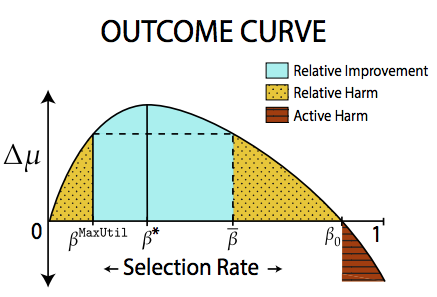
The Outcome Curve

Possible areas
| Area | Description |
|---|---|
| Active Harm | Expected change in credit score of an individual is negative |
| Stagnation | Expected change in credit score of an individual is 0 |
| Improvement | Expected change in credit score of an individual is positive |
Possible areas
| Area | Description |
|---|---|
| Relative Harm | Expected change in credit score of an individual is less than if the selection policy had been to maximize profit |
| Relative Improvement | Expected change in credit score of an individual is better than if the selection policy had been to maximize profit |
For those interested in more of an explanation of the equations, see Appendix
Causality
"Correlation doesn't imply causation"
But what is causation?
If we can understand what causes unfair behavior, then we can take steps to mitigate it.
Basic idea: if a sensitive attribute has no causal influence on prediction, don't use it.
But how do we model causation?
Causal Graphs
Solution: build causal graphs of your problem
Problem: causality cannot be inferred from observational data
Observational data can only show correlations
For causal information we have to do experiments. (But that is often not ethical.)
Example with Causal Graphs
Example: Law school success
Task: given GPA score and LSAT (law school entry exam), predict grades after one year in law school: FYA (first year average)
Additionally two sensitive attributes: race and gender
Example with Causal Graphs
Two possible graphs

Counterfactual Fairness
$U$: set of all unobserved background variables
$P(\hat{y}_{s=i}(U) = 1|x, s=i)=P(\hat{y}_{s=j}(U) = 1|x, s=i)$
$i, j \in \{0, 1\}$
$\hat{y}_{s=k}$: prediction in the counterfactual world where $s=k$
practical consequence: $\hat{y}$ is counterfactually fair if it does not causally depend (as defined by the causal model) on $s$ or any descendants of $s$.
Related idea: fairness based on similarity
- First define a distance metric on your datapoints (i.e. how similar are the datapoints)
- Can be just Euclidean distance but is usually something else (because of different scales)
Pre-processing based on similarity
- An individual is then considered to be unfairly treated if it is treated differently than its "neighbours".
- For any data point we can check how many of the $k$ nearest neighbours have the same class label as that data point
- If the percentage is under a certain threshold then there was discrimination against the individual corresponding to that data point.
- Then: flip the class labels of those data points where the class label is considered unfair
Considering similarity during training
Alternative idea:
- a classifier is fair if and only if the predictive distributions for any two data points are at least as similar
as the two points themselves
- (according to a given similarity measure for distributions and a given similarity measure for data points)
Considering similarity during training
- Needed similarity measure for distributions
- Then add fairness condition as additional loss term to optimization loss
Appendix
Introduction
This paper is about acknowledging a feedback loop.
Credit decisions are ultimately more than just whether or not you get a loan. It also affects an applicant's credit history is they're accepted for a loan that they can't repay.
$$ u(x) = u_+ p(x) + u_- ( 1 - p(x) ) $$
Where $u_+$ is the profit of a repaid loan
and $u_-$ is the loss on an unpaid loan
$$ U(\tau) = \sum_{j \in \{A,B\}} g_j \sum_{x \in \mathcal{X}} \tau_j(x) \pi_j(x)u(x) $$
where $g_j$ is the fraction of the total population
Where $c_+$ isa constant gain in credit score if loan repaid
and $c_-$ is a constant loss in the case of an unpaid loan
$$ \Delta\mu_j(\tau) = \sum_{x \in \mathcal{X}} \pi_j(x) \tau_j(x) \Delta (x) $$
Where $\Delta(x)$ as defined on the slide before is the expected change in score of an individual with score $x$
Fairness Criteria
This paper considers 3
- Maximizing Utility
- Demographic Parity
- Equality of Opportunity
Maximizing Utility
This is the null constraint. The bank solely focusses on utility (earning money)Demographic Parity
Equal selection rates for groups $A$ and $B$Equality of Opportunity
Equal True Positive Rates across the 2 groups$$TPR_A(\tau_A) = TPR_B(\tau_B)$$
Where
$$ TPR_j(\tau) = \frac{\sum_{x \in \mathcal{X}} \pi_j (x) p(x) \tau)x)}{\sum_{x \in \mathcal{X}} \pi_j(x) p(x)} $$
The Outcome Curve

Possible areas
| Area | Description |
|---|---|
| Active Harm | $\Delta \mu_j (\tau_j) < 0$ |
| Stagnation | $\Delta \mu_j (\tau_j) = 0$ |
| Improvement | $\Delta \mu_j (\tau_j) > 0$ |
| Relative Harm | $\Delta \mu_j (\tau_j) < \Delta \mu_j (\tau^{\text{MAXUTIL}})$ |
| Relative Improvement | $\Delta_j (\tau_j) > \Delta \mu_j (\tau^{\text{MAXUTIL}})$ |
Selection Rates
$$ \beta_j = \sum_{x \in \mathcal{X}} \pi_j(x) \tau_j(x) $$| Selection Rate | Description |
|---|---|
| $\beta^{\text{MAXUTIL}}$ | The selection rate under max util |
| $\beta^*$ | selection rate such that $\Delta \mu_A$ is maximized |
| $\bar{\beta}$ | the outcome complement of the MaxUtil selection rate, $\Delta \mu_A r_{\pi_A}^{-1}(\bar{\beta}) = \Delta \mu_A (r_{\pi_A}^{-1} (\beta^{\text{MAXUTIL}}))$ with $\bar{\beta} > \beta^{\text{MAXUTIL}}$ |
| $\beta_0$ | the harm threshold, such that $\Delta \mu_A r_{\pi_A}^{-1} (\beta_0) = 0$ |
Findings/Results
Under the assumption $\frac{u_-}{u_+} < \frac{c_-}{c_+}$ which means that the risk to the bank is greater than the risk to the individual$$ 0 \leq \Delta \mu (\tau^{\text{MAXUTIL}}) \leq \Delta \mu^* $$
Under the assumption $\beta_{A}^{\text{MAXUTIL}} < \bar{\beta}$ and $\beta_{A}^{\text{MAXUTIL}} < \beta_{B}^{MAXUTIL}$ there exists population proportions $g_0 < g_1 < 1$ such that for all $g_A \in [g_0,g_1]$, $\beta_{A}^{\text{MAXUTIL}} < \beta_{A}^{\text{DEMPARITY}} < \bar{\beta}$